Forecasting Crypto Prices using Deep Learning (Time Series #3)

[CA]: Time Series #3 - Forecasting Cryptocurrency Prices (Time Series) using Deep Learning (PyTorch, Tensorflow/Keras & darts)

CA=Competence Afternoon

Series is 3 parts, 1. Part One - Decomposing & Working with Time Series (theoretical) () 2. Part Two - Predicting Stock Prices (Time Series) using classical Machine Learning () 3. Part Three -Forecasting Cryptocurrency Prices (Time Series) using Deep Learning (PyTorch, Tensorflow/Keras & darts) ()

Predicting Time Series 📈

Today we’ll move on from analyzing and using simple models to predict time series to using advanced models and using libraries that simplifies some of the work.

To be able to predict the data we must understand it and we’ll make a minor analysis.

Installation & Imports

from IPython.display import clear_output
!pip install -U pandas_datareader
!pip install plotly
!pip install pytorch-lightning
!pip install -U darts
!pip install matplotlib==3.1.3
!pip install pyyaml==5.4.1

clear_output()

import pandas as pd # data processing, CSV file I/O (e.g. pd.read_csv)
import numpy as np  # linear algebra
import pandas_datareader as pdr
import seaborn as sns
from darts import TimeSeries

from datetime import datetime

/usr/local/lib/python3.7/dist-packages/distributed/config.py:20: YAMLLoadWarning: calling yaml.load() without Loader=... is deprecated, as the default Loader is unsafe. Please read https://msg.pyyaml.org/load for full details.
  defaults = yaml.load(f)

def get_btc_close() -> pd.Series:
  return pdr.get_data_yahoo('BTC-USD')['Close']

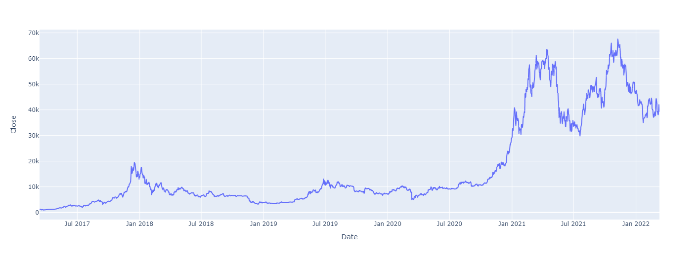
df = get_btc_close()
print(df.head())

df.plot(y='Close', backend='plotly')

Date
2017-03-12    1221.380005
2017-03-13    1231.920044
2017-03-14    1240.000000
2017-03-15    1249.609985
2017-03-16    1187.810059
Name: Close, dtype: float64

Show Plotly Chart (code cell only visible in active notebook)

Data Wrangling & Transformation

Last time we built \(t_0 .. t_x\) time steps. This is bad because it makes our memory consumption explode.
How can we solve this?

generators meme

Generators

We can solve it by batching the data and building the batch on-the-fly. This is achieved through use of generators and the yield keyword in Python.
A lot like a lazy sequence really.

See image 👇

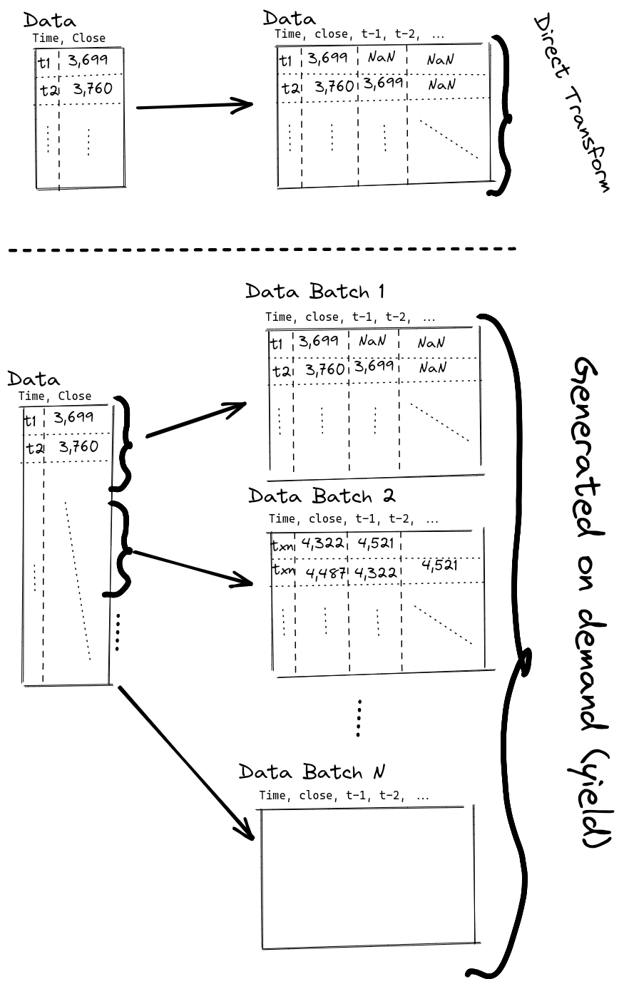
By using this kind of batching we can generate a subset of the dataset at a time which in turn does not blow our memory through the roof and to the moon.

How would we implement this in practise?
Turns out it’s not that hard. You can do it by hand with usual np.ndarray, list or anything, but I choose to use torch.utils.data.Dataset which is the PyTorch dataset. This means that we’ll have data in the same format that we’d feed into our PyTorch-model. 🥳

First we need to implement torch.utils.data.Dataset which is simple in Python;

import torch

class TimeseriesDataset(torch.utils.data.Dataset):
  def __init__(self):
    pass

Then we need to instantiate it by saving X and y, and a seq_len which is our window-size.

Using the self keyword we’ll save the value as a class value.
Instead of typing our input we could’ve wrapped X and y with torch.tensor to make sure they’re the correct type. But as a fan of types I really prefer this approach, rather than band-aiding it inside the __init__.

class TimeseriesDataset(torch.utils.data.Dataset):
    def __init__(self, X: torch.tensor, y: torch.tensor, seq_len: int=1):
        self.X = X
        self.y = y
        self.seq_len = seq_len

We’re still missing some crucial methods to make this work in the end, even if Python don’t complain (hey, it’s Python - what did I expect? ¯_ (ツ)_/¯).

__len__ needs to be implemented to let downstream task consume the dataset. Without a length you won’t know how much data there is.

class TimeseriesDataset(torch.utils.data.Dataset):
    def __init__(self, X: torch.tensor, y: torch.tensor, seq_len: int=1):
        self.X = X
        self.y = y
        self.seq_len = seq_len
    
    def __len__(self) -> int:
        return self.X.__len__() - (self.seq_len - 1)

self.X.__len__() - (self.seq_len - 1) <– What is this sorcery?

Remember from part #2 where we built our history we had to use pd.DataFrame.dropna, the same has to be done here which means our final dataset is a little bit less than len(X).

Now there’s a single piece left, __getitem__(self, index) which fetches the element(s).
For our use-case we wish to window/slide the data, so we’ll fetch a slice, [a:b], as X and the future element as y.

class TimeseriesDataset(torch.utils.data.Dataset):
    def __init__(self, X: torch.tensor, y: torch.tensor, seq_len: int=1):
        self.X = X
        self.y = y
        self.seq_len = seq_len
    
    def __len__(self) -> int:
        return self.X.__len__() - (self.seq_len - 1)
    
    def __getitem__(self, index):
        return (self.X[index:index + self.seq_len], self.y[index + self.seq_len - 1])

That’s it, simple right? 🥳

Let’s test it and validate that this works.

ℹ️ torch.roll is the equivalent of pd.DataFrame.shift.
ℹ️ torch.utils.data.DataLoader is PyTorch loader that provides simple batching, multiprocessing and much more automatically!

tensor_close = torch.tensor(df)
train_dataset = TimeseriesDataset(tensor_close[:-1], tensor_close.roll(-1)[:-1], seq_len=7)
train_loader = torch.utils.data.DataLoader(train_dataset, batch_size=128, shuffle=False)
train_loader

<torch.utils.data.dataloader.DataLoader at 0x7f98210aeb90>

And validating the input

for batch in train_loader:
    print(f"X: {batch[0][:2]}")
    print(f"y: {batch[1][:2]}")
    break

X: tensor([[1221.3800, 1231.9200, 1240.0000, 1249.6100, 1187.8101, 1100.2300,
          973.8180],
        [1231.9200, 1240.0000, 1249.6100, 1187.8101, 1100.2300,  973.8180,
         1036.7400]], dtype=torch.float64)
y: tensor([1036.7400, 1054.2300], dtype=torch.float64)

Seems like the math is on point the first element in y is the same as the final element in the second X-tensor. And the second y is nowhere to be found (as that’d be final in the third X-tensor).

Using a library made for Time Series - darts

Darts allows us to use State-of-the-Art models very easily, just like scikit-learn has a interface for most Machine Learning models.

df.head()

Date
2017-03-12    1221.380005
2017-03-13    1231.920044
2017-03-14    1240.000000
2017-03-15    1249.609985
2017-03-16    1187.810059
Name: Close, dtype: float64

Then using TimeSeries.from_* we can load the data into TimeSeries.

ts = TimeSeries.from_series(df)

train, val = ts.split_before(0.8)
train.plot(label="Train")
val.plot(label="Validation")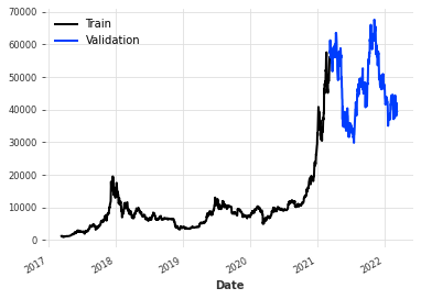

In darts there’s a plethora of utility functions such as fill_missing_values & add_holidays.
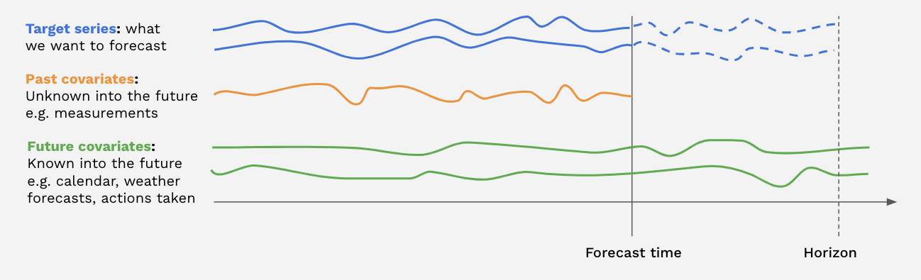
darts also make it really simple to do - Multivariate Forecasting.
- Forecasting with Covariates

💡 Multivariate Forecasting is when you include multiple variables with their history. Predicting a single signal is called Univariate Forecasting.

💡 Covariates are other things that are known like holiday, I think the image below is very telling.

covariates-darts

Using SHAP (A game theoretic approach to explain the output of any machine learning model.) you can identify which covariates that affects the result the most. But I’ll leave that for another time.

from darts.dataprocessing.transformers import Scaler
from darts.models import NBEATSModel, RNNModel, RandomForest, TCNModel, Prophet
from darts.utils.statistics import check_seasonality, plot_acf
from darts.metrics import mape

First we need to scale the data, most models expect the data to be in a good format and having increasingly overly large numbers can be hard to work with.

darts provide a Scaler which is like a Transform from scikit-learn.

scaler = Scaler()

train_scaled = scaler.fit_transform(train)
train_scaled.plot()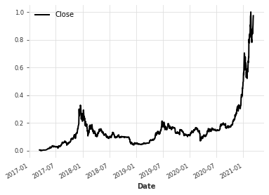

Let’s train a model on this data.
NBEATS is a really good model and as such let’s use it.

What does the parameters do?

param	action
input_chunk_length	This is the “lookback window” of the model- i.e., how many time steps of history the neural network takes as input to produce its output in a forward pass.
output_chunk_length	This is the “forward window” of the model - i.e., how many time steps of future values the neural network outputs in a forward pass.
random_state	Just as in scikit-learn and other toolkits we wish to have reproducible results, hence we set random_state

from darts.models import NBEATSModel, RNNModel, Prophet, RandomForest, TCNModel, TFTModel

model = NBEATSModel(input_chunk_length=7, output_chunk_length=1, random_state=42,)
model.fit(train_scaled, epochs=10)

[2022-03-11 14:31:44,193] INFO | darts.models.forecasting.torch_forecasting_model | Train dataset contains 1453 samples.
[2022-03-11 14:31:44,193] INFO | darts.models.forecasting.torch_forecasting_model | Train dataset contains 1453 samples.
[2022-03-11 14:31:44,663] INFO | darts.models.forecasting.torch_forecasting_model | Time series values are 64-bits; casting model to float64.
[2022-03-11 14:31:44,663] INFO | darts.models.forecasting.torch_forecasting_model | Time series values are 64-bits; casting model to float64.
GPU available: True, used: False
TPU available: False, using: 0 TPU cores
IPU available: False, using: 0 IPUs
/usr/local/lib/python3.7/dist-packages/pytorch_lightning/trainer/trainer.py:1585: UserWarning:

GPU available but not used. Set the gpus flag in your trainer `Trainer(gpus=1)` or script `--gpus=1`.


  | Name      | Type       | Params
-----------------------------------------
0 | criterion | MSELoss    | 0     
1 | stacks    | ModuleList | 6.1 M 
-----------------------------------------
6.1 M     Trainable params
1.3 K     Non-trainable params
6.1 M     Total params
48.490    Total estimated model params size (MB)

<darts.models.forecasting.nbeats.NBEATSModel at 0x7f980cde79d0>

Now that the model is trained we wish to do a historical_forecasts to validate how it would’ve done on the validation data.

Let’s go ahead!

val_scaled = scaler.transform(val)

%%capture
preds = model.historical_forecasts(
    val_scaled, start=0.1, forecast_horizon=1, retrain=False
)

# scale back:
preds = scaler.inverse_transform(preds)

val.plot(label="actual")
preds.plot(label="predicted")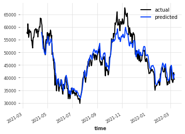

Try using different forecasting, like forecast_horizon=7.
To make it even more interesting you should reshape the model to use output_chunk_length=7, which should mean it’s better at predicting further into the future as that target has been “developed” during training.

Try new models like RNNModel, Prophet (by Facebook), TCNModel (Temporal Convolutional Neural Network), TCTModel (Temporal Fusion Transformer) or our old buddy RandomForest.

Find more models in the docs.

PyTorch

We should not only have fun with pre-built libraries but it’d be nice to try building this by hand using PyTorch.

I’ll dump the code, but walk it through right below on what and why.

First we’ll define our class

class RNNModel(pl.LightningModule):

Which in our case is a pytorch-lightning (pl) one, pl is a very thin wrapper on top of PyTorch that automate some mundane tasks, but still makes it easy to configure them by hand as I’ll show.

Then we’ll define our __init__:

class RNNModel(pl.LightningModule):
  def __init__(self, 
                 n_features, 
                 hidden_size, 
                 seq_len, 
                 batch_size,
                 num_layers, 
                 dropout, 
                 learning_rate,
                 criterion):
        super(RNNModel, self).__init__()
        self.n_features = n_features
        self.hidden_size = hidden_size
        self.seq_len = seq_len
        self.batch_size = batch_size
        self.num_layers = num_layers
        self.dropout = dropout
        self.criterion = criterion
        self.learning_rate = learning_rate

        self.lstm = nn.LSTM(input_size=n_features, 
                            hidden_size=hidden_size,
                            num_layers=num_layers, 
                            dropout=dropout, 
                            batch_first=True)
        self.linear = nn.Linear(hidden_size, 1)

That’s a lot to chew! 😅
Let’s walk it through,

argument	what it does
hidden_size	width of the RNN (e.g. cells)
num_layers	the number of layers of RNNs
dropout	the dropout probability between the layers in the RNN, requires >= 2 layers
seq_len	the window/history size
learning_rate	the learning rate
criterion	the loss function

Seems OK right?
In the __init__ we defined all our parts required to run the neural network, but we need to define how to run it. That’s what we define forward to do, and the backward-pass is automatically done for us.

def forward(self, x):
  # lstm_out = (batch_size, seq_len, hidden_size)
  lstm_out, _ = self.lstm(x)
  y_pred = self.linear(lstm_out[:,-1])
  return y_pred

First we run our data through the LSTM, then our linear/dense layer to retrieve a single output. Sounds good?

And that’s really all that’s needed for a PyTorch-model. But because I chose to use pytorch-lightning to simplify our training loop we need a little more:

def configure_optimizers(self):
  return torch.optim.Adam(self.parameters(), lr=self.learning_rate)

def predict_step(self, batch, batch_idx, dataloader_idx):
  x,y = batch
  return self(x)

def training_step(self, batch, batch_idx):
  x, y = batch
  y_hat = self(x)
  loss = self.criterion(y_hat, y)
  self.log('train_loss', loss)
  
  return loss

First we define our optimizer to be Adam in configure_optimizers.
Then we define how to predict, e.g. only splitting our batch. predict_step is defined by default to simply run forward which does not fit our dataloaders.
Finally we define training_step which explains how to run training. On top of this I define testing_step and validation_step to do the exact same except for the logging.

💡the self.log will automatically allow us to log everything with Tensorboard – cool right?

RNNModel PyTorch

Run the two cells below that contains the pl.LightningModule and our PyTorch Dataset.

import pytorch_lightning as pl
from torch import nn
import torch
import torch.nn.functional as F
from torch.autograd import Variable

class RNNModel(pl.LightningModule):
    def __init__(self, 
                 hidden_size, 
                 seq_len, 
                 batch_size,
                 num_layers, 
                 dropout, 
                 learning_rate,
                 criterion):
        super(RNNModel, self).__init__()
        self.hidden_size = hidden_size
        self.seq_len = seq_len
        self.batch_size = batch_size
        self.num_layers = num_layers
        self.dropout = dropout
        self.criterion = criterion
        self.learning_rate = learning_rate

        self.lstm = nn.LSTM(input_size=1, 
                            hidden_size=hidden_size,
                            num_layers=num_layers, 
                            dropout=dropout, 
                            batch_first=True)
        self.linear = nn.Linear(hidden_size, 1)
        
    def forward(self, x):
        # lstm_out = (batch_size, seq_len, hidden_size)
        lstm_out, _ = self.lstm(x)
        y_pred = self.linear(lstm_out[:,-1])
        return y_pred

    def configure_optimizers(self):
        return torch.optim.Adam(self.parameters(), lr=self.learning_rate)

    def predict_step(self, batch, batch_idx, dataloader_idx=0):
      x,y = batch
      return self(x)

    def training_step(self, batch, batch_idx):
        x, y = batch
        y_hat = self(x)
        loss = self.criterion(y_hat, y)
        self.log('train_loss', loss)
        
        return loss

    def validation_step(self, batch, batch_idx):
        x, y = batch
        y_hat = self(x)
        loss = self.criterion(y_hat, y)
        self.log('val_loss', loss)
        
        return loss
    
    def test_step(self, batch, batch_idx):
        x, y = batch
        y_hat = self(x)
        loss = self.criterion(y_hat, y)
        self.log('test_loss', loss)

        return loss

class TimeseriesDataset(torch.utils.data.Dataset):   
    '''
    Custom Dataset subclass. 
    Serves as input to DataLoader to transform X 
      into sequence data using rolling window. 
    DataLoader using this dataset will output batches 
      of `(batch_size, seq_len, n_features)` shape.
    Suitable as an input to RNNs. 
    '''
    def __init__(self, X: np.ndarray, y: np.ndarray, seq_len: int = 7):
        self.X = torch.tensor(X).float()
        self.y = torch.tensor(y).float()
        self.seq_len = seq_len

    def __len__(self):
        return self.X.__len__() - (self.seq_len - 1)

    def __getitem__(self, index):
        return (self.X[index:index+self.seq_len], self.y[index+self.seq_len-1])

The DataModule

This step is not really a requirement but rather a show-case of how to create a pl.LightningDataModule which contains all your code to validate different models simpler as you only need to supply your datamodule to do everything.

Let me walk us through it.

class BitcoinDataModule(pl.LightningDataModule):
    
    def __init__(self, seq_len = 7, batch_size = 128, num_workers=0):
      # add arguments

Defining our class and __init__.

We then need to define our setup which loads the data and our dataloaders, which is done in the following sense:

def setup(self, stage=None):
  X = df[:-1]
  y = df.shift(-1)[:-1]

  X_cv, X_test, y_cv, y_test = train_test_split(
      X, y, test_size=0.2, shuffle=False
  )

  X_train, X_val, y_train, y_val = train_test_split(
      X_cv, y_cv, test_size=0.25, shuffle=False
  )

  preprocessing = StandardScaler()
  preprocessing.fit(X_train)

  self.X_train = preprocessing.transform(X_train)
  self.y_train =  preprocessing.transform(y_train).reshape((-1, 1))
  self.X_val = preprocessing.transform(X_val)
  self.y_val = preprocessing.transform(y_val).reshape((-1, 1))

def train_dataloader(self):
  train_dataset = TimeseriesDataset(self.X_train, 
                                    self.y_train, 
                                    seq_len=self.seq_len)
  train_loader = DataLoader(train_dataset, 
                            batch_size = self.batch_size, 
                            shuffle = False, 
                            num_workers = self.num_workers)
  
  return train_loader

def val_dataloader(self):
  # repeat train_dataloader

This is rather simple, even if it’s a lot of code.

DataModule definition

from sklearn.model_selection import train_test_split
from sklearn.preprocessing import StandardScaler
from torch.utils.data import DataLoader

class BitcoinDataModule(pl.LightningDataModule):
    '''
    PyTorch Lighting DataModule subclass:
    https://pytorch-lightning.readthedocs.io/en/latest/datamodules.html

    Serves the purpose of aggregating all data loading and processing work in one place.
    '''
    
    def __init__(self, seq_len = 7, batch_size = 128, num_workers=0):
        super().__init__()
        self.seq_len = seq_len
        self.batch_size = batch_size
        self.num_workers = num_workers
        self.X_train = None
        self.y_train = None
        self.X_val = None
        self.y_val = None
        self.X_test = None
        self.X_test = None
        self.preprocessing = None

    def prepare_data(self):
        pass

    def setup(self, stage=None):
        if stage == 'fit' and self.X_train is not None:
            return 
        if stage == 'test' and self.X_test is not None:
            return
        if stage is None and self.X_train is not None and self.X_test is not None:  
            return
        
        X = df[:-1].to_numpy().reshape(-1, 1)
        y = df.shift(-1)[:-1].to_numpy().reshape(-1, 1)

        X_cv, X_test, y_cv, y_test = train_test_split(
            X, y, test_size=0.2, shuffle=False
        )
    
        X_train, X_val, y_train, y_val = train_test_split(
            X_cv, y_cv, test_size=0.25, shuffle=False
        )

        preprocessing = StandardScaler()
        preprocessing.fit(X_cv)

        if stage == 'fit' or stage is None:
            self.X_train = preprocessing.transform(X_train)
            self.y_train =  preprocessing.transform(y_train).reshape((-1, 1))
            self.X_val = preprocessing.transform(X_val)
            self.y_val = preprocessing.transform(y_val).reshape((-1, 1))

        if stage == 'test' or stage is None:
            self.X_test = preprocessing.transform(X_test)
            self.y_test = preprocessing.transform(y_test).reshape((-1, 1))
        

    def train_dataloader(self):
        train_dataset = TimeseriesDataset(self.X_train, 
                                          self.y_train, 
                                          seq_len=self.seq_len)
        train_loader = DataLoader(train_dataset, 
                                  batch_size = self.batch_size, 
                                  shuffle = False, 
                                  num_workers = self.num_workers)
        
        return train_loader

    def val_dataloader(self):
        val_dataset = TimeseriesDataset(self.X_val, 
                                        self.y_val, 
                                        seq_len=self.seq_len)
        val_loader = DataLoader(val_dataset, 
                                batch_size = self.batch_size, 
                                shuffle = False, 
                                num_workers = self.num_workers)

        return val_loader

    def test_dataloader(self):
        test_dataset = TimeseriesDataset(self.X_test, 
                                         self.y_test, 
                                         seq_len=self.seq_len)
        test_loader = DataLoader(test_dataset, 
                                 batch_size = self.batch_size, 
                                 shuffle = False, 
                                 num_workers = self.num_workers)

        return test_loader

Training our Model

Let’s move on to the fun part! First we define our input values such as dropout, criterion and more.

seq_len = 7
batch_size = 256
criterion = nn.MSELoss()
max_epochs = 300
hidden_size = 56
num_layers = 2
dropout = 0.2
learning_rate = 1e-3

Then we define our trainer, model & dm and in the end do a fit.

trainer = pl.Trainer(max_epochs=max_epochs, gpus=1, log_every_n_steps=4)

model = RNNModel(
    hidden_size = hidden_size,
    seq_len = seq_len,
    batch_size = batch_size,
    criterion = criterion,
    num_layers = num_layers,
    dropout = dropout,
    learning_rate = learning_rate
)

dm = BitcoinDataModule(
    seq_len = seq_len,
    batch_size = batch_size
)

trainer.fit(model, dm)
clear_output()
trainer.test(model, dm)

LOCAL_RANK: 0 - CUDA_VISIBLE_DEVICES: [0]

--------------------------------------------------------------------------------
DATALOADER:0 TEST RESULTS
{'test_loss': 3.8363118171691895}
--------------------------------------------------------------------------------

[{'test_loss': 3.8363118171691895}]

How does this look in the TensorBoard?

%load_ext tensorboard
%tensorboard --logdir=lightning_logs/

And let’s validate how good our predictions are. Please note that we trained for 300 epochs with not a lot of data, running perhaps 500 should yield bettwer results.
But I’ll leave that for you to play around with 😉

predictions_all_batches = trainer.predict(model, dataloaders=dm.val_dataloader())

LOCAL_RANK: 0 - CUDA_VISIBLE_DEVICES: [0]

preds = torch.cat(predictions_all_batches)

true = []
for _, y_true in dm.val_dataloader():
  true += y_true

true = torch.cat(true)

pd.DataFrame({'Preds': preds.flatten(), 'True': true.flatten()}).plot(backend="plotly")

Show Plotly Chart (code cell only visible in active notebook)

TensorFlow - Keras

Let’s do it the Keras way!

df.head()

Date
2017-03-12    1221.380005
2017-03-13    1231.920044
2017-03-14    1240.000000
2017-03-15    1249.609985
2017-03-16    1187.810059
Name: Close, dtype: float64

First we wish to scale our data to make sure it’s easier for our model to learn its weights.

Then we wish to create our Dataset, luckily tf.keras has a utility function called timeseries_dataset_from_array which solves this for us. Creating the data we wish for!

One could also look at tf.keras.TimeseriesGenerator for a even better approach. But for now let’s keep it easy.

import tensorflow as tf

seq_len = 7
scaler = StandardScaler()
data_scaled = scaler.fit_transform(np.array(df).reshape(-1, 1))

def make_dataset(data: pd.Series):
  data = np.array(data, dtype=np.float32)
  return tf.keras.utils.timeseries_dataset_from_array(
      data=data,
      targets=np.roll(data, -seq_len), # move into future
      sequence_length=seq_len,
      sequence_stride=1,
      shuffle=False,
      batch_size=32)

train, val = train_test_split(data_scaled, test_size=0.2, shuffle=False)

ds_train = make_dataset(train)
ds_val = make_dataset(val)

ds_train

<BatchDataset element_spec=(TensorSpec(shape=(None, None, 1), dtype=tf.float32, name=None), TensorSpec(shape=(None, 1), dtype=tf.float32, name=None))>

Let’s validate that the input looks good

for example_inputs, example_labels in ds_train.take(1):
  print(f'Inputs shape (batch, time, features): {example_inputs.shape} - {example_inputs[0]}')
  print(f'Labels shape (batch, time, features): {example_labels.shape} - {example_labels[0]}')

Inputs shape (batch, time, features): (32, 7, 1) - [[-0.90802824]
 [-0.90742284]
 [-0.90695876]
 [-0.9064068 ]
 [-0.90995634]
 [-0.9149866 ]
 [-0.92224723]]
Labels shape (batch, time, features): (32, 1) - [-0.9186332]

data_scaled[:8]

array([[-0.90802824],
       [-0.90742286],
       [-0.90695878],
       [-0.90640682],
       [-0.90995636],
       [-0.91498662],
       [-0.92224724],
       [-0.91863324]])

The 8th element does indeed correspond to the label printed above, as expected. The 1-7th ones also correspond to the input data.

Superb! 🥳

Now we’d like to build a very simple Baseline which simply predicts the previous timestep. Just as with PyTorch we need to define our class (tf.keras.Model), __init__ and finally call which is similar to PyTorch’s forward.

class Baseline(tf.keras.Model):
  def __init__(self):
    super().__init__()

  def call(self, inputs):
    return inputs[:, -1]

💡
Sequential class: Sequential groups a linear stack of layers into a tf.keras.Model.
Model class: Model group’s layers into an object with training and inference features.

Sequential is the simplest form with linear stack of layers and is restricted in what’s possible, meanwhile Model we can instantiate a Model with the Functional API which allows us to form arbitrary graphs of layers and share features/data between multiple layers.

TL;DR Model is very similar to how PyTorch operates and Sequential is a simplification that’s useful for simpler problems.

After defining our Baseline we wish to compile our model as it’s graciously called in tf.keras. When calling compile we define our metrics, optimizer & loss-function.

It’s simple and it makes sense based on what we’ve seen previously in PyTorch.
As our baseline don’t need to train we’ll simply run evaluate to see how good it performs!

baseline = Baseline()

baseline.compile(loss=tf.losses.MeanSquaredError(),
                 metrics=[tf.metrics.MeanAbsoluteError()])

val_performance = {}
val_performance['Baseline'] = baseline.evaluate(ds_val)

12/12 [==============================] - 1s 11ms/step - loss: 0.0135 - mean_absolute_error: 0.0774

To make sure we aren’t blinded by the metrics (MAE, mean absolute error) we’ll plot the result to validate how it looks compared to the true data.

preds = baseline.predict(ds_val)
y_val = np.concatenate([y for (x,y) in list(ds_val)])

preds.shape, y_val.shape

((360, 1), (360, 1))

pd.DataFrame({"Preds": preds.flatten(), "True": y_val.flatten()}).plot(backend="plotly")

Show Plotly Chart (code cell only visible in active notebook)

😮…that’s really good. But that’s also to be expected as we’re always predicting the same as the previous day!

How about we try a little bit more complex model using a linear network?
We’ll add a method called compile_and_fit which takes a model, training/validation data and adds a EarlyStopping criteria that stops if we don’t improve enough.

We’ll use tf.keras.Sequential to make the simplest type of network where we’ll just chain layers together.

from tqdm.keras import TqdmCallback

linear = tf.keras.Sequential([
    tf.keras.layers.Dense(units=7),
    tf.keras.layers.Dense(units=1)
])

MAX_EPOCHS = 20

def compile_and_fit(model, ds_train, ds_val, patience=2):
  early_stopping = tf.keras.callbacks.EarlyStopping(monitor='val_loss',
                                                    patience=patience,
                                                    mode='min')

  model.compile(loss=tf.losses.MeanSquaredError(),
                optimizer=tf.optimizers.Adam(),
                metrics=[tf.metrics.MeanAbsoluteError()])

  history = model.fit(ds_train, epochs=MAX_EPOCHS,
                      validation_data=ds_val,
                      callbacks=[early_stopping, TqdmCallback(verbose=1)], verbose=0)
  return history

history = compile_and_fit(linear, ds_train, ds_val)

preds = linear.predict(ds_val)

pd.DataFrame({"Preds": preds[:,-1,:].flatten(), "True": y_val.flatten()}).plot(backend="plotly")

Show Plotly Chart (code cell only visible in active notebook)

The predictions looks good, but it seems VERY overfitted as we follow the lines pretty much perfectly. It very much looks like our Baseline, and that’s a issue I’d say. We wish to generalize better.

multi_step_dense = tf.keras.Sequential([
    # Shape: (time, features) => (time*features)
    tf.keras.layers.Flatten(input_shape=(7,)),
    tf.keras.layers.Dense(units=32, activation='relu'),
    tf.keras.layers.Dense(units=32, activation='relu'),
    tf.keras.layers.Dense(units=1),
    # Add back the time dimension.
    # Shape: (outputs) => (1, outputs)
    tf.keras.layers.Reshape([1, -1]),
])

history = compile_and_fit(multi_step_dense, ds_train, ds_val)

preds = multi_step_dense.predict(ds_val)

pd.DataFrame({"Preds": preds.flatten(), "True": y_val.flatten()}).plot(backend="plotly")

Show Plotly Chart (code cell only visible in active notebook)

This result is worse and better. 🤷

➕ Better generalization
➖ Worst case predictions are worse

Let’s try LSTM as we did in PyTorch! 🤖

lstm_model = tf.keras.models.Sequential([
    # Shape [batch, time, features] => [batch, time, lstm_units]
    tf.keras.layers.LSTM(32),
    # Shape => [batch, time, features]
    tf.keras.layers.Dense(units=1)
])

MAX_EPOCHS = 50
history = compile_and_fit(lstm_model, ds_train, ds_val, patience=10)

preds = lstm_model.predict(ds_val)
print(preds.shape)
pd.DataFrame({"Preds": preds.flatten(), "True": y_val.flatten()}).plot(backend="plotly")

(360, 1)

Show Plotly Chart (code cell only visible in active notebook)

Once again we find a trend-line, this time a bit smoother. But it doesn’t follow the values perfectly and the MAE is higher.

💡 Quick-fixes: Try more epochs, and LSTMs usually require more data so having a larger dataset might help.

Play around! Do what you wish to do! This is easy to improve upon, and real fun! 💪

---

To learn more about Time Series and how one can analyze them please view the other parts,

1. Part One - Decomposing & Working with Time Series (theoretical)
2. Part Two - Predicting Stock Prices (Time Series) using classical Machine Learning
3. Part Three -Forecasting Cryptocurrency Prices (Time Series) using Deep Learning (PyTorch, Tensorflow/Keras & darts)

---

Extra Material

Do you like the fast.ai-approach? Then make sure to check out the awesome tsai! It contains a lot of the SotA-models.

Do you wish for another PyTorch approach? Then check out pytorch-forecasting which is also available in lightning-flash.
Do you wish for a third (and really awesome ❗) approach with PyTorch? Then make sure to research neuralforecast which actually includes the latest models such as Informer.

That’s all for these three posts, have a great time exploring!

~Hampus Londögård