2019-02-04 AFRY NLP Competence Meeting: Text Classification IMDB

I’ve set a goal to create one blog post per Competence Meeting I’ve held at AFRY to spread the knowledge further. This goal will also grab all the older meetings, my hope is that I’ll be finished before summer 2020, but we’ll see.

Introduction

Most of my Competence Meetings take place in the form of Jupyter Notebooks (.ipynb). Notebooks are awesome as they allow us to:

Mix and match markdown & code-blocks
Keep the state of the program, i.e. very explorative

This is really good in combination with the workshop-format that we usually have. Using services such as Google Colab one can take the file and open it in the browser and run it there. This means that we don’t need any downloads and pretty often we also have a speed gain because the node used is faster than a laptop with its GPU.

Let’s get on to the competence evening.

Text Classification

Today we’ll go through text classification, what it is, how it is used and how to make it yourself while trying to keep have a great mix of both theory and practical use. Text classification is just what the name suggest, a way to classify texts. Let it be spam or reviews, you train it and it’ll predict what class the text belongs to.

A good baseline

To have a good baseline is incredibly important in Machine Learning. In summary you want the following

Simple model to predict outcome
Use this model to compare your new, more complex model to

This is to be able to know what progress you’re making. You don’t want to do anything more complex without any gains.

One pretty common simple baseline is just to pick a random class as prediction.

Classes & Features

What is a class and feature?

Features are the input to the model, you can see a machine learning system as a "consumer" of features. You can view this as a cookie monster consuming cookies and then he says if they taste good or bad. He has the input, cookie, that can be a feature. He then has a output, class, that is good/bad. Repeat this a lot of times and you can retrieve statistics if Cookie Y is good or bad.

To generalize this system we would divide the feature into multiple feature, like what ingredients the cookie contains. So instead of saying this is a "Chocolate Chip Cookie" we know tell the system the features are:

chocolate: yes
sugar:yes
honey:no
oat:no
cinnamon: no
sweet: yes
sour: no\"

. In numerical input it would translate to something as [1,1,0,0,0,1,0].

One-Hot-Encoding - how we represent features & classes

As shown in the translation to numerical vectors we don’t represent words as actual words. We always use numbers, often we even use something called One-Hot-Encoding.

One-Hot-Encoding means that we have an array of one 1 and the rest is 0s. This is to optimize math performed by the GPU (or CPU).

Using the example of Good & Bad cookies with the extension of Decent we will One-Hot-Encode these as the following

Good   = [1,0,0]
Bad    = [0,1,0]
Decent = [0,0,1]

The same is applied to our features. If you’re using a framework (such as Keras) it is pretty common that they include an method to do this, or even that it is done automatically for you.

Back to text classification

To classify a text we do what is called an sentiment analysis meaning that we try to estimate the sentiment polarity of a text body. In the first part of this workshop we’ll be assuming that there’s only two sentiments, Negative and Positive. Then we can express this as the following classification problem:

Feature: String body
Class:   Bad|Good

The output, Classes, are easy to One-Hot-Encode but how do we succesfully One-Hot-Encode a string? A character can be seen as a class but is that really something we can learn from? To solve this we need to preprocess our input somehow.

Preprocessing

Preprocessing is an incredibly important part of Machine Learning. Combining preprocessing with Data Mining is actually around 70% of the workload (IBM) when developing models through the CRISP-DM. From my experience this is true.

Having good data and finding the most important features is incredibly important to have a competent system. In this task we need to preprocess the text to simplify the learning process for our system. We will do the following:

Clean the text
Vectorize the texts into numerical vectors

Cleaning the text

Why do we need to clean the text? It is to remove weird stuff & outliers. If we have the text I'm a cat.we want to simplify this into [i'm, a, cat] or even [im, a, cat].

Removing data such as non-alphabetical characters and the letter case makes more data look a like and reduces the dimension of our input – this simplifies the learning of the system. But removing features can be bad also, if someone writes in all CAPS we can guess that they’re angry. But let’s take that later.

import regex as re


def clean_text(text):
    \"\"\"
    Applies some pre-processing on the given text.

    Steps :
    - Removing punctuation
    - Lowering text
    \"\"\"
    
    # remove the characters [\\], ['] and [\"]
    text = re.sub(r\"\\\\\", \"\", text)    
    text = re.sub(r\"\\'\", \"\", text)    # Extra: Is regex needed? Other ways to accomplish this.
    text = re.sub(r\"\\\"\", \"\", text)
    # replace all non alphanumeric with space 
    text = re.sub(r\"\\W+\", \" \", text)
    # text = re.sub(r\"<.+?>\", \" \", text) # <br></br>hej<br></br>
    
    # Extra: How would we go ahead and remove HTML? Time to learn some Regex!
    
    return text.strip().lower()
clean_text(\"Wow, we can clean text now. Isn't that amazing!?\").split()

Vectorization

Now that we can extract text we need to be able to input it to the system. We have to vectorize it. In this part we’ll vectorize each word as a number. The simplest approach to this is using Bag of Words (BOW).

Bag of Words creates a list of words which is called the Dictionary. The Dictionary is just a list of the words from the training data.

Training data: [\"ÅF is a big company\", \"ÅF making future\"]
--> Dictionary: [ÅF, is, a, big, company, making, future]

New text: \"ÅF company is a future company\" --> [1,1,1,0,2,0,1]

Our new text is vectorized on top of the dictionary. You take the dictionary and replace the words position with the count of it that is found in the new text.

Finalizing the preprocessing

We can actually do some more things to improve the system which I won’t go into detail about (read the code). We remove stop-words and so on.

from sklearn.feature_extraction.text import CountVectorizer


training_texts = [
    \"ÅF is a big company\", 
    \"ÅF making future\"
]

test_texts = [
    \"ÅF company is a future company\"
]

# this is the vectorizer
vectorizer = CountVectorizer(
    stop_words=\"english\",    # Removes english stop words (such as 'a', 'is' and so on.)
    preprocessor=clean_text  # Customized preprocessor
)

# fit the vectorizer on the training text
vectorizer.fit(training_texts)

# get the vectorizer's vocabulary
inv_vocab = {v: k for k, v in vectorizer.vocabulary_.items()}
vocabulary = [inv_vocab[i] for i in range(len(inv_vocab))]

# vectorization example
pd.DataFrame(
    data=vectorizer.transform(test_texts).toarray(),
    index=[\"Test sentence\"],
    columns=vocabulary
)

Let’s do something fun out of this!

To begin with we need data. Luckily I know a perfect dataset for this – the IMDB movie reviews from stanford. This is a widely used dataset throughout Sentiment Analysis. The data contains 50 000 reviews where 50 % is positive and the rest negative. First we fetch a dataset. Download this file and unpack it (into aclImdb) if the first code-snippet was unsuccessful.

import os
import numpy as np

def load_train_test_imdb_data(data_dir):
    \"\"\"
    Loads the IMDB train/test datasets from a folder path.
    Input:
    data_dir: path to the \"aclImdb\" folder.
    
    Returns:
    train/test datasets as pandas dataframes.
    \"\"\"

    data = {}
    for split in [\"train\", \"test\"]:
        data[split] = []
        for sentiment in [\"neg\", \"pos\"]:
            score = 1 if sentiment == \"pos\" else 0

            path = os.path.join(data_dir, split, sentiment)
            file_names = os.listdir(path)
            for f_name in file_names:
                with open(os.path.join(path, f_name), \"r\") as f:
                    review = f.read()
                    data[split].append([review, score])
  
    # We shuffle the data to make sure we don't train on sorted data. This results in some bad training.
    np.random.shuffle(data[\"train\"])        
    data[\"train\"] = pd.DataFrame(data[\"train\"],
                                 columns=['text', 'sentiment'])

    np.random.shuffle(data[\"test\"])
    data[\"test\"] = pd.DataFrame(data[\"test\"],
                                columns=['text', 'sentiment'])

    return data[\"train\"], data[\"test\"]
train_data, test_data = load_train_test_imdb_data(
    data_dir=\"aclImdb/\")

Let’s create our classifier

We now have a dataset that we have successfully partitioned into a dictionary so that we can use it for our classifier.

Do you see an issue with our baseline right now?

…As mentioned we want to only have important features to simplify training. Right now we have an enormous amount of features, our BOW-approach result in an 80 000-dimensional vector. Because of this we must use simple algorithms that learn fast & easy, e.g. Linear SVM, Naive Bayes or Logistic Regression.

Let’s create some code that actually let’s us train a Linear SVM!

from sklearn.metrics import accuracy_score
from sklearn.svm import LinearSVC


# Transform each text into a vector of word counts
vectorizer = CountVectorizer(stop_words=\"english\",
                             preprocessor=clean_text)

training_features = vectorizer.fit_transform(train_data[\"text\"])    
test_features = vectorizer.transform(test_data[\"text\"])

# Training
model = LinearSVC()
model.fit(training_features, train_data[\"sentiment\"])
y_pred = model.predict(test_features)

# Evaluation
acc = accuracy_score(test_data[\"sentiment\"], y_pred)

print(\"Accuracy on the IMDB dataset: {:.2f}\".format(acc*100))

Comparison to state-of-the-art

Our accuracy is somewhere around 83.5-84 % which is really good! With this simple model and incredibly simplistic feature extraction we achieve a really high amount of correct answer! Comparing this to state-of-the-art we’re around 11 percent units beneat (~95% accuracy achieved here).

Incredible right? Exciting!? For me it is at least!

How do we improve from here?

Improving the model

We have some huge improvements to make outside of fine-tuning, so we’ll skip the fine-tuning from now.

The first step is to improve our vectorization.

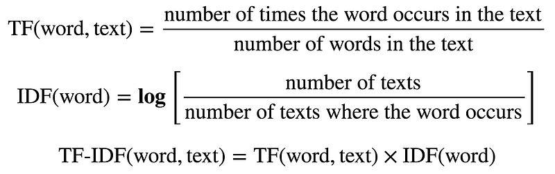
TF-IDF

If you were at first friday ((ÅF?)) you have heard about TF-IDF earlier. TF-IDF stands for Term Frequence-Inverse Document Frequency and is a measurement that aims to fight imbalances in texts.

In our vectorization step we look at the word-count meaning that we’ll have some biases to how much a word is present, the longer the text the more the bias. To reduce this we can take the word-count divided by the total amount of words in the text (TF). We also want to downscale the words that are incredibly frequent such as stop words and topic-related words, and upscale unusual words somewhat, e.g.glamorous might not be frequent but it is important to the text most likely. We use IDF for this. We then take these two and combine.

Implementation details

This is actually really easy to do as sklearn already has a finished TfIdfVectorizer so all we have to do is to replace the CountVectorizer. Let’s see how it goes!

from sklearn.svm import LinearSVC
from sklearn.metrics import accuracy_score
from sklearn.feature_extraction.text import TfidfVectorizer


# Transform each text into a vector of word counts
vectorizer = TfidfVectorizer(stop_words=\"english\",
                             preprocessor=clean_text)

training_features = vectorizer.fit_transform(train_data[\"text\"])    
test_features = vectorizer.transform(test_data[\"text\"])

# Training
model = LinearSVC()
model.fit(training_features, train_data[\"sentiment\"])
y_pred = model.predict(test_features)

# Evaluation
acc = accuracy_score(test_data[\"sentiment\"], y_pred)

print(\"Accuracy on the IMDB dataset: {:.2f}\".format(acc*100))

# Extra: Implement our own TfIdfVectorizer.

Conclusion of TF-IDF

The TfIdVectorizer improved our scoring with 2 percent units, that’s incredible for such an easy improvement!

This for me shows how important it is to understand the data and what is important. You really need to grasp how to extract the important and what tools are available.

But let’s not stop here, lets reiterate and improve further.

What is the next natural step? Context I believe. During my master-thesis on spell correction of Street Names it was very obvious how important context is to increase the models understanding. Unfortunately we couldn’t use the context of a sentence in the thesis (as of the nature of street names) but here we can!

Use of context

Words by themself prove some meaning but sometimes they’re used in a negated sense, e.g. not good. Good in itself would most likely be positive but if we can get the context around the word we can be more sure about in what manner it is applied.

We call this N-grams where N is equal to the amount of words taken into consideration for each word. Using bigrams (N=2) we get the following:

companies often use corporate bs => [companies, often, use, slogans, (companies, often), (often,use), (use,slogans)]

Sometimes you include a start & ending word so that it would be (\\t, companies) and (slogans, \\r) or such. In this case as we are not finetuning we won’t go into that. We’ll keep it simple.

The all-mighty sklearn TfIdfVectorizer actually already have included N-gram support using the parameter ngram_range=(1, N). So let’s make it simple for us and make use of that!

from sklearn.svm import LinearSVC
from sklearn.metrics import accuracy_score
from sklearn.feature_extraction.text import TfidfVectorizer


# Transform each text into a vector of word counts
vectorizer = TfidfVectorizer(ngram_range=(1, 2),
                            strip_accents='ascii',
                            max_df=0.98)

training_features = vectorizer.fit_transform(train_data[\"text\"])    
test_features = vectorizer.transform(test_data[\"text\"])

# Training
model = LinearSVC()
model.fit(training_features, train_data[\"sentiment\"])
y_pred = model.predict(test_features)

# Evaluation
acc = accuracy_score(test_data[\"sentiment\"], y_pred)

print(\"Accuracy on the IMDB dataset: {:.2f}\".format(acc*100))

Conclusion of N-gram

Once again we see a massive improvement. We’re almost touching 89 % now! That’s just a mere 6 percent units below state-of-the-art. What can we do to improve now?

Some possible improvements for you to try!

Use a custom threshold to reduce the dimensions
Play around with the ngram_range (don’t forget a threshold if you do this)
Improve the preprocessing

# Try some fun things here if you want too :)

Conclusion of phase 1

We have created a strong baseline for text classification with great accuracy for its simplicity. The following steps has been done

First a simple preprocessing step which is of great importance. We have to remember to not make it to complex, the complexity of preprocessing is like an evil circle in the end. In our case we remove punctuations, stopwords and lower the case.
Secondly we vectorize the data to make it readable by the system. A classifier requires numerical features. For this we had a TfIdfVectorizer that computes frequency of words while downsampling words that are to common & upsampling unusual words.
Finally we added N-gram to the model to increase the understanding of the sentence by supplying context.

Phase 2

How do we improve from here? TF-IDF has its cons and pros. Some of the cons are that they:

Don’t account for any kind of positioning at all
The dimensions are ridiculous large
They can’t capture semantics.

Improvements upon this is made by using neural networks and word embeddings.

Word Embeddings

Word Embeddings & Neural Networks are where we left off. By change our model to instead utilize these two concepts we can improve the accuracy once again.

Word Embeddings

Word Embeddings (WE) are actually a type of Neural Network. It uses embedding to create the model. I quickly explained WE during my presentation on Summarization and how to build a great summarizer. Today we’ll go a little more into depth.

To begin with I’ll take the most common example, WE lets us do the following arithmetiric with words:

King - Man + Woman = Queen

This is, in my opinion, completely amazing and fascinating. How does this work? Where do I learn more? Those are my first thoughts. In fact the theory is pretty basic until you get to the nittygritty details, as with most things.

WE is built on the concept ot learn how words are related to eachother. What company do a word have? To make the example more complex we can redefine this too the following: A is to B what C is to D.

Currently there is three "big" models that are widely used. The first one Word2Vec (Mikolov et al 2013), the second is GloVe (MIT MIT, Pennington et al 2014) and the final one is fastText (facebook).

We will look into how you can achieve this without Deep Learning / Neural Networks unlike the models mentioned.

Step 1: How to represent words in a numerical vector

The first thing we have to do to actually understand/achieve word embeddings is to represent words in a numerical vector. In relation to this a quick explanation of sparse & dense representations would be great. Read more in detail at Wikipedia: Sparse Matrix

Sparse representation is when we represent something very sparsely. It tells us that the points in the space is very few in regards to the dimensions and that most elements are empty. Think one-hot-encoding.

A Dense representation in comparison has few dimensions in comparison to possible values and most elements are filled. Think of something continuous.

The most simple way to represent words in a numerical vector is something we touched earlier, by one-hot-encoding them, i.e. a sparse representation.

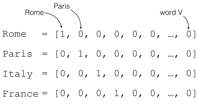Source :(Marco Bonzanini, 2017) (Source: Marco Bonzanini, 2017)

Because of how languages are structured having one-hot-encoding means that we will have an incredibly sparse matrix (can be good) but it will have an enormous amount of dimensions (bad).

On top of this how would we go ahead and measure the distance between words? Normally one would use the cosine similarity but if we have a one-hot-encoding all the words would be orthogonal against eachother meaning that the dot-product will be zero.

Creating a dense representation however would indeed capture similarity as we could make use of cosine-similarity and more. Introducing Word2Vec.

Step 2: Word2Vec, representing data densely

The goal of Word2Vec, at least to my understanding, is to actually predict the context of a word. Or in other words we learn embeddings by prediciting the context of the word. The context here being the same definition as in N-grams. Word2Vec uses shallow neural network to learn word vectors so that each word is good at predicting its own contexts (more about his in Skip-Grams) and how to predict a word given a context (more about this in CBOW).

Skip-gram

Skip-gram very simplified is when you train on the N-grams but without the real word. 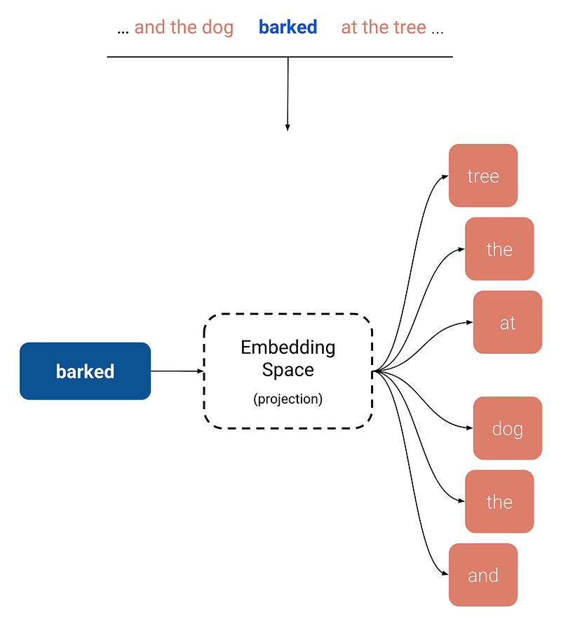alt text

As of now we have empirical results showing how this technique is very successful at learning the meaning of the words. On top of this the embedding that we get has both direction of semantic and syntatic meaning that are exposed in example such as King - Man....

Another example would be: Vector(Madrid) - Vector(Spain) + Vector(Sweden) ~ Vector(Stockholm)

So how do the arithmetic of words actually work?

I won’t go into details (some complicated math, see Gittens et al) but if we assume the following to be true:

All words are distributed uniformly
The embedding model is linear
The conditional distributions of words are indepedent

Then we can prove that the embedding of the paraphrase of a set of words is obtained by taking the sum over the embeddings of all of the individual words.

Using this result it’s easy to show how the famous man-woman, king-queen relationship works.

Extra note: You can show this then by havingn King and Queen having the same Male-Femalerelationship as the King then is the paraphrase of the set of words {Queen, X}

I want to note that these assumptions are not 100 percent accurate. In reality word distributions are thought to follow Zipf’s law.

GloVe

A year after Word2Vec was a fact to the world the scientist decided to reiterate again. This time we got GloVe. GloVe tried to improve upon Word2Vec by that given a word its relationship(s) can be recovered from co-occurence statistics of a large corpus. GloVe is expensive and memory hungry, but it’s only one load so the issue isn’t that big. Nitty bitty details

fastText

With fastText one of the biggest problems is solved, both GloVe and Word2Vec only learn embeddings of word of the vocabulary. Because of this we can’t find an embedding for a word that isn’t in the dictionary.

Bojanowski et al solved this by learning the word embeddings using subword information. To summarize fastText learns embeddings of character n-grams instead.

The simple way

A simple approach to create your own word embeddings without a neural network is by factorizing a co-occurence matrix using SVD (singular-value-decomposition). As mentioned Word2Vec is barely a neural network as it has no hidden layers nor an y non-linearities. GloVe factorizes a co-occurense matrix while gaining even better results.

I highly recommend you to go check this blog out: https://multithreaded.stitchfix.com/blog/2017/10/18/stop-using-word2vec/ by Stitch Fix. An awesome read and we can go implement this too!